Flow Matching
Flow matching is a highly effective mathematical framework for generative modeling. It serves as an alternative to Diffusion Models and provides a more intuitive, efficient way to train Continuous Normalizing Flows (CNFs).
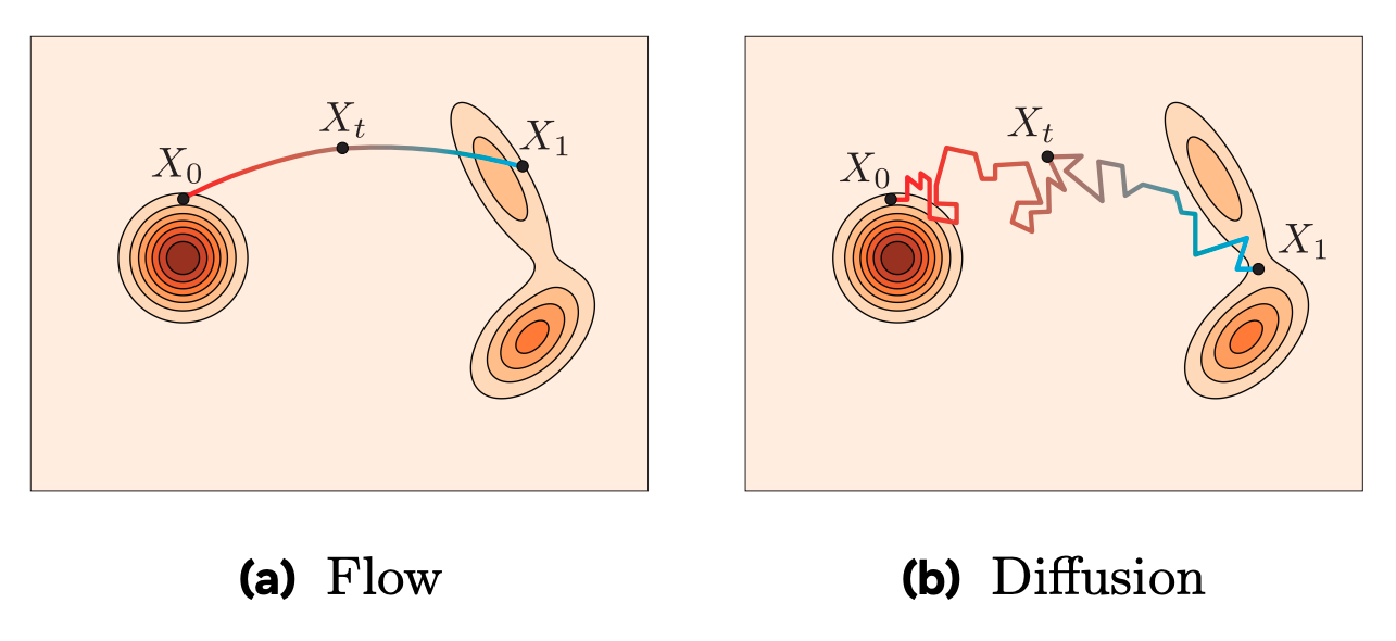
At its core, flow matching aims to learn a vector field that gradually transforms a simple, known probability distribution (like standard Gaussian noise) into a complex, unknown distribution (like a dataset of high-resolution images).
Here is a detailed breakdown of the mathematics behind flow matching.
1. The Core Objective: Probability Paths and Vector Fields
In generative modeling, we want to transform a simple base distribution, \(p_0(x)\) (typically noise), into our target data distribution, \(p_1(x)\).
Flow matching constructs a continuous probability density path, \(p_t(x)\), where \(t \in [0, 1]\). At \(t=0\), we have noise; at \(t=1\), we have data.
This probability path is governed by a time-dependent vector field, \(v_t(x)\). You can think of this vector field as the "wind" that blows the probability mass from the noise distribution into the shape of the data distribution. The relationship between the probability path and the vector field is defined by the continuity equation:
\[\frac{\partial}{\partial t} p_t(x) + \nabla \cdot (p_t(x) v_t(x)) = 0\]
If we know the vector field \(v_t(x)\), we can generate new data by drawing a sample \(x_0 \sim p_0(x)\) and solving an Ordinary Differential Equation (ODE) over time \(t\) from 0 to 1:
\[\frac{d}{dt}x_t = v_t(x_t)\]
Our machine learning goal is to train a neural network, \(v_\theta(x, t)\), with parameters \(\theta\), to approximate this true vector field \(v_t(x)\).
2. The Marginal Flow Matching Objective (The Intractable Problem)
Ideally, we would just train our neural network to match the true vector field directly using a simple Mean Squared Error (MSE) loss:
\[\mathcal{L}_{FM}(\theta) = \mathbb{E}_{t \sim \mathcal{U}(0,1), x \sim p_t(x)} [||v_\theta(x, t) - v_t(x)||^2]\]
However, this objective is intractable. In practice, we do not know the true marginal vector field \(v_t(x)\), nor do we know the intermediate marginal probability distributions \(p_t(x)\), because calculating them requires integrating over the entire, complex dataset.
3. The Breakthrough: Conditional Flow Matching (CFM)
The primary mathematical breakthrough of Flow Matching (introduced by Lipman et al., 2023) is a technique that makes this tractable.
Instead of trying to match the *marginal* vector field of the entire dataset, we define a conditional vector field, \(u_t(x\|z)\), and a conditional probability path, \(p_t(x\|z)\), based on a conditioning variable \(z\). Typically, \(z\) is just a single data point from our dataset, \(x_1 \sim p_1(x)\).
By conditioning on a single data point \(x_1\), we define exactly how a single particle of noise should travel to become that specific data point.
The Conditional Flow Matching loss is defined as:
\[\mathcal{L}_{CFM}(\theta) = \mathbb{E}_{t \sim \mathcal{U}(0,1), x_1 \sim p_1(x), x \sim p_t(x|x_1)} [||v_\theta(x, t) - u_t(x|x_1)||^2]\]
Why does this work? Through a mathematical property, it can be proven that the gradients of the conditional loss are identical to the gradients of the intractable marginal loss: \(\nabla_\theta \mathcal{L}_{CFM}(\theta) = \nabla_\theta \mathcal{L}_{FM}(\theta)\). By minimizing the tractable conditional loss, we are implicitly minimizing the true marginal loss.
4. Optimal Transport (OT) Flow Matching
Because we are conditioning on individual data points, we have total freedom to design *how* the noise travels to the data point. The most popular and efficient choice is to make the paths straight lines. This is often referred to as Optimal Transport (OT) Flow Matching or Rectified Flow.
If we sample noise \(x_0 \sim \mathcal{N}(0, I)\) and a data point \(x_1\), we can define the path between them as linear interpolation:
\[x_t = t x_1 + (1 - t) x_0\]
Because the path is a straight line, the target vector field (the derivative with respect to time) becomes incredibly simple—it is just the constant velocity required to get from \(x_0\) to \(x_1\):
\[u_t(x|x_1, x_0) = \frac{d}{dt} x_t = x_1 - x_0\]
The loss function simplifies beautifully to:
\[\mathcal{L}_{OT-CFM}(\theta) = \mathbb{E}_{t \sim \mathcal{U}(0,1), x_0 \sim p_0, x_1 \sim p_1} [||v_\theta(x_t, t) - (x_1 - x_0)||^2]\]
During training, the neural network predicts the direction \((x_1 - x_0)\) given the intermediate noisy point \(x_t\) and the time \(t\). During inference, we start with pure noise, step through the ODE solver guided by the network's velocity predictions, and arrive at a newly generated data point.
