Generative Adversarial Network (GAN)

A generative adversarial network, or GAN, is a generative model: after training, it turns a handful of random numbers into a new sample that looks like its training data, here a handwritten digit that nobody wrote. It was proposed in 2014 as a simple and appealing idea: train the generator against a second network that learns to tell its drawings from real ones. Making that idea work in practice took years of fixes. This note follows that path, from the idea and why it should work, to the three problems that got in the way, vanishing gradients, non-convergence and mode collapse, and the fixes that made GANs practical.

Every number quoted comes from our own models, trained on MNIST (60,000 training digits of 28 × 28 pixels, scaled to \([-1, 1]\)) with fixed seeds. Our generator is the MNIST generator of InfoGAN: 64 random numbers go through two fully connected layers (1,024 and 128 · 7 · 7 units) and two transposed convolutions (to 64 channels at 14 × 14, then one channel at 28 × 28), with batch normalization and ReLU, and a tanh at the end. Our critic mirrors it: two strided convolutions (64 and 128 channels) and two fully connected layers (1,024 units, then one output), with leaky ReLU and no batch normalization, so that its score for a picture depends on that picture alone. Both train with Adam (learning rate \(2 \times 10^{-4}\), \(\beta_1 = 0.5\), \(\beta_2 = 0.999\)) on batches of 128, for 20 epochs or 9,360 steps.

The task: no answer key

We want random numbers in and a picture out that looks like a real digit: sharp, and of every kind, in the proportions of the data. Write the generator as a function \(G\) from a noise vector \(z\), 64 numbers drawn from the standard normal distribution, to a picture \(G(z)\). Nothing says which noise should become which picture, so no drawing has a target to be compared with. A model that pairs each training image with codes, like the Variational Autoencoder (VAE), can grade its drawing against that image; a GAN has no such pairs.

Could pixel distance to real pictures grade "looks real"? Take our running three, test digit 1134, and the same three moved three pixels to the right. Both are real threes, yet their pixel distance (the Euclidean distance between their 784 values in \([0, 1]\)) is 9.92, and only 56% of their ink overlaps. Their average, a blurred double-stroke three, is 4.96 from each, half as far. So pixel distance ranks a blur that nobody would write closer to the two real threes than they are to each other. It measures the wrong thing: looking real is not the same as being close, pixel by pixel, to some real picture.

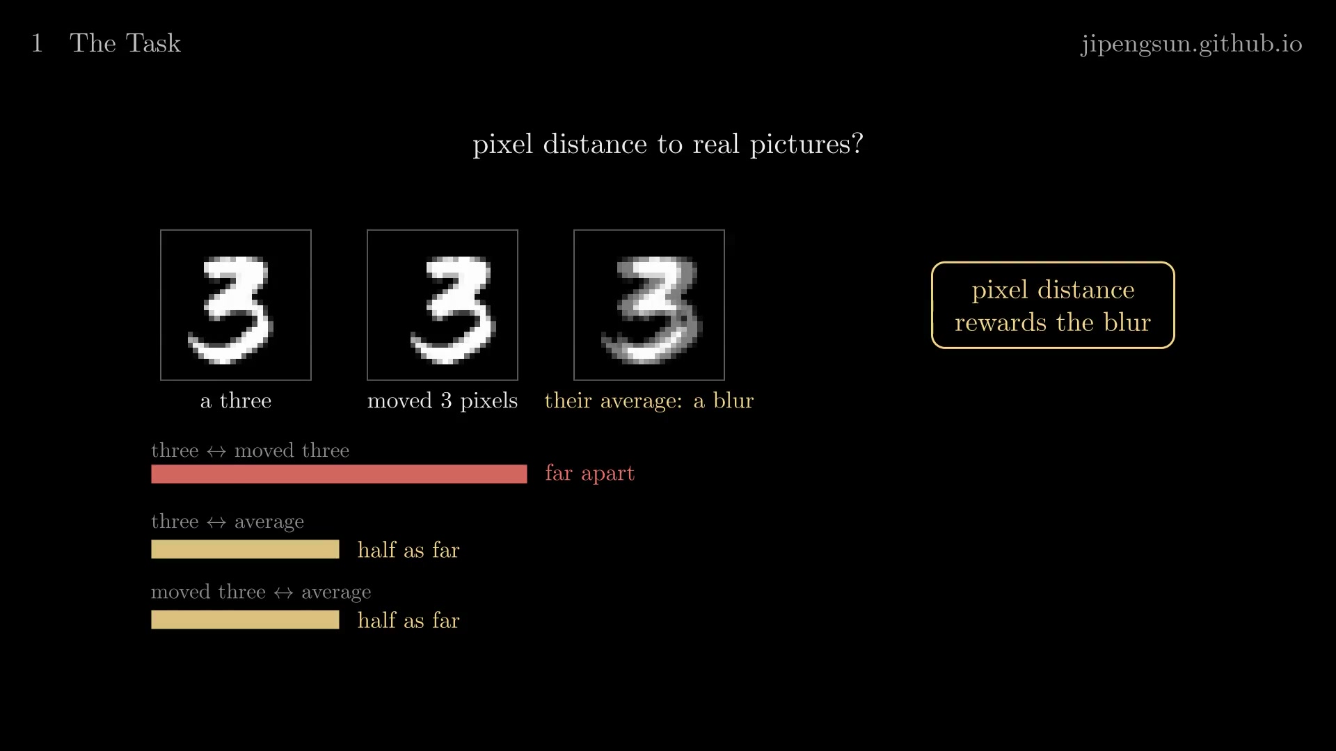
Figure 1. Pixel distance measures the wrong thing: a three and the same three moved three pixels are far apart, while their blurred average sits half as far from each.

A learned judge: the critic

Looking real has no formula, but telling real pictures from fakes is a classification problem, the kind of task neural networks do well (the note on Discriminative vs. Generative Models describes that side). So a GAN learns its grade. A second network, the discriminator, or critic, \(D\), maps a picture \(x\) to \(D(x) \in (0, 1)\), the probability that \(x\) is real. Its training labels come free: 1 for pictures drawn from the data, 0 for the generator's drawings. No digit labels are needed, so the same recipe trains on faces or rooms.

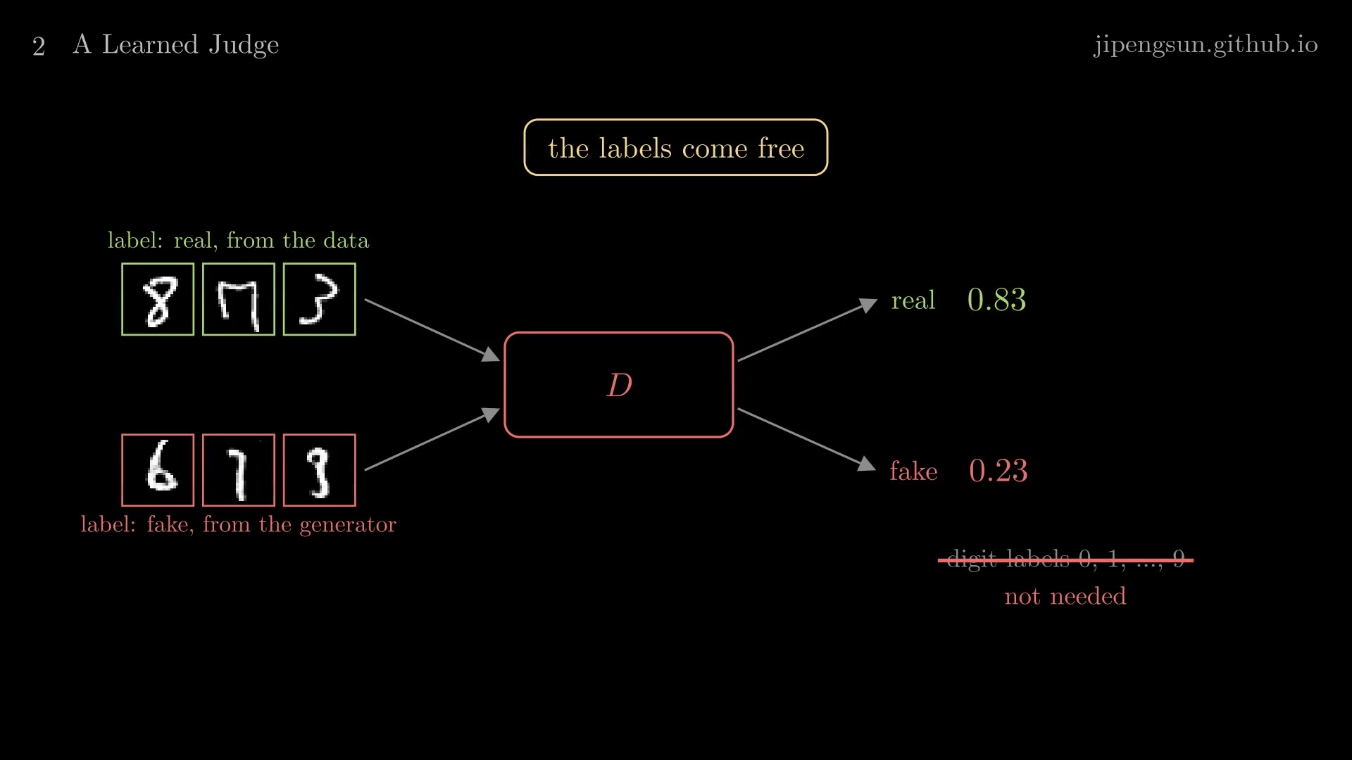
Figure 2. The critic learns its grade from free labels: real for pictures from the data, fake for the generator's drawings. No digit labels are needed.

The critic's loss is the binary cross-entropy of these labels,

\[L_D = -\,\mathbb E_{x \sim p_{\text{data}}}\big[\log D(x)\big] \;-\; \mathbb E_{z}\big[\log\big(1 - D(G(z))\big)\big],\]

where \(p_{\text{data}}\) is the distribution of the real digits and the second expectation runs over noise vectors \(z\). It is small when real pictures score near 1 and fakes near 0.

Two networks, one game

The generator learns to make the critic call its fakes real, while the critic learns to catch them: the two are adversaries. The original paper wrote the generator's goal as minimizing \(\mathbb E_z[\log(1 - D(G(z)))]\), the critic's own fake term with the opposite aim, which makes training a two-player minimax game. We train the generator with the variant the same paper recommends,

\[L_G = -\,\mathbb E_{z}\big[\log D(G(z))\big],\]

which is smallest, zero, only when the critic scores every fake 1, as if it were real, so the generator's steps push its fakes' scores toward 1; the section on vanishing gradients shows why this variant matters. The two take turns: one small step of the critic on a batch of 128 real digits and 128 fakes, then one small step of the generator. The generator's gradient reaches its weights through the critic: differentiating \(L_G\) with respect to a fake's pixels says, for every pixel, which way would look more real to the critic, and backpropagation carries that into the generator's weights.

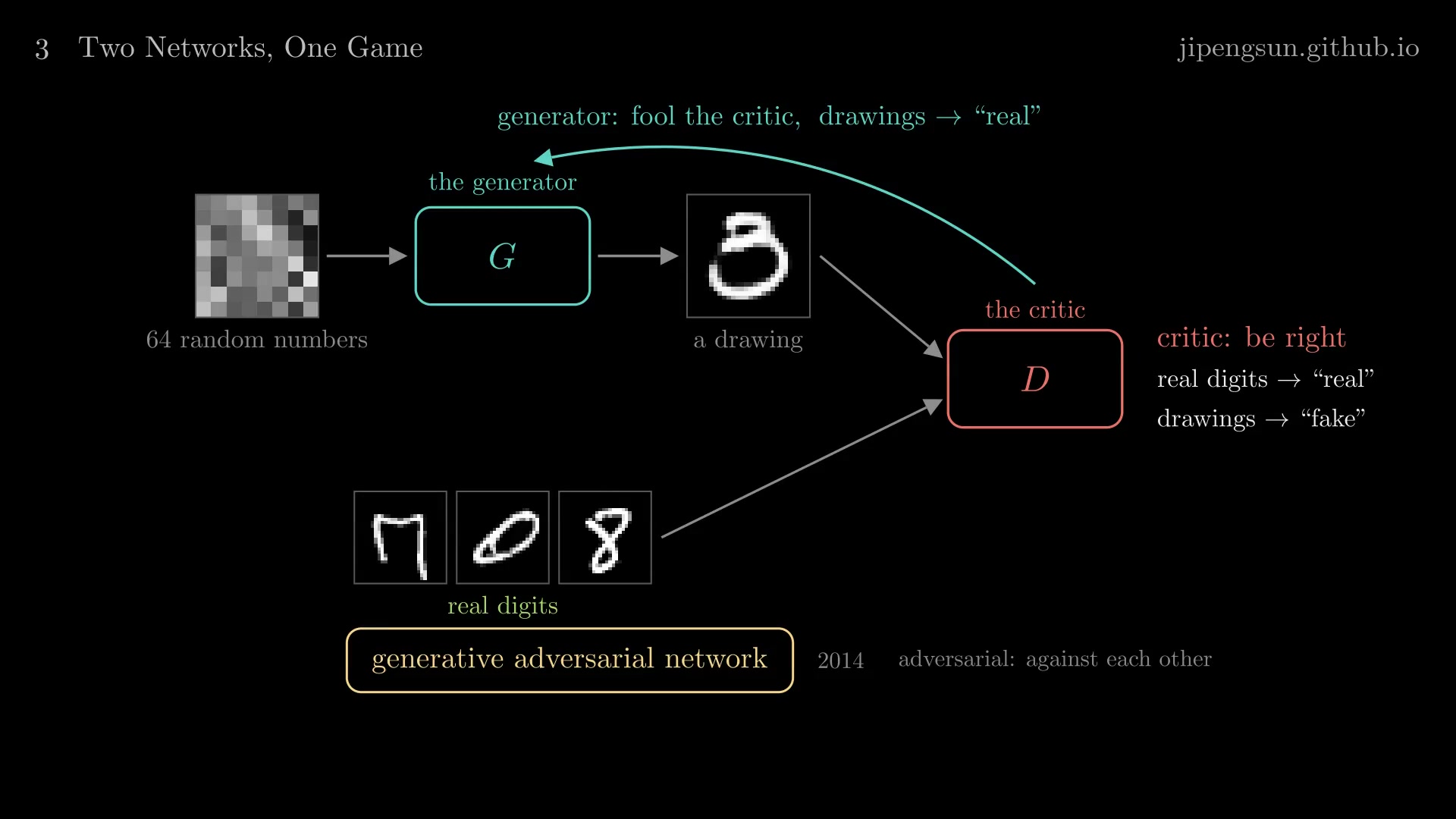
Figure 3. Opposite goals: the critic wants to be right, real digits called real and drawings called fake; the generator wants to fool it, so its drawings must look more and more like real digits. Hence the name: two networks working against each other.

Here is one real step of ours, step 3,163 of a run continued from the state at step 3,000. Before the critic's step, its mean score was 0.645 on the batch's real digits and 0.374 on its fakes; the step moved them to 0.669 and 0.350; the generator's step then raised the fakes' mean to 0.431. We picked this step as the clearest of 200: in each half, at least 74% of the examples moved the same way as the batch. On most steps, Adam's momentum moves the real and fake scores up or down together, while the gap between them still widens. Turn after turn, our generator's drawings went from a flat gray at step 0, through high-contrast textures (step 100) and strokes (step 300), to rough digits by step 1,000 and clean ones by step 2,000.

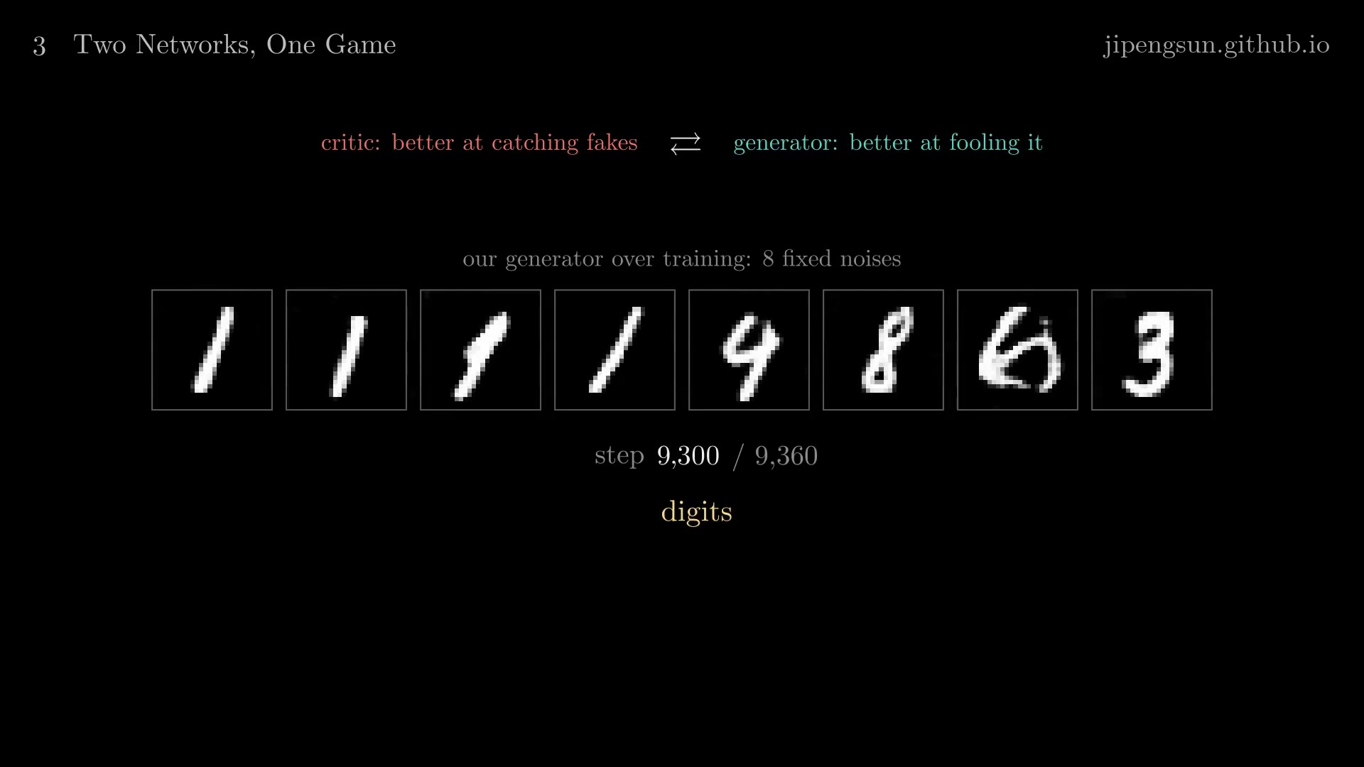
Figure 4. Our generator's drawings for eight fixed noises at step 9,300. Turn after turn, noise became strokes, then digits.

Why it should work

Suppose the generator is fixed and its drawings follow a distribution \(p_g\). The critic's loss is then \(-\int \big[p_{\text{data}}(x) \log D(x) + p_g(x) \log(1 - D(x))\big]\, dx\), and since \(a \log D + b \log(1 - D)\) is largest at \(D = a/(a+b)\), the best critic is

\[D^*(x) = \frac{p_{\text{data}}(x)}{p_{\text{data}}(x) + p_g(x)},\]

the share of real pictures among all the pictures that look like \(x\). With digit kinds standing in for pictures: if the real data has 10% of each digit and the generator draws 30% threes, 2% fives and 8.5% of each other digit, the best critic scores a three \(10/(10+30) = 0.25\), a five \(10/(10+2) = 0.83\), and each of the rest \(10/18.5 = 0.54\). Moving drawings toward higher scores means fewer threes and more fives, until every kind appears as often as in the data, where every score is one half.

The exact statement follows from plugging \(D^*\) into the minimax objective. With the mixture \(m = (p_{\text{data}} + p_g)/2\), we have \(D^* = p_{\text{data}}/(2m)\) and \(1 - D^* = p_g/(2m)\), so

\[\begin{aligned} \mathbb E_{p_{\text{data}}}\big[\log D^*\big] + \mathbb E_{p_g}\big[\log(1 - D^*)\big] &= -\log 4 + \mathrm{KL}(p_{\text{data}} \,\Vert\, m) + \mathrm{KL}(p_g \,\Vert\, m) \\ &= -\log 4 + 2\,\mathrm{JSD}(p_{\text{data}} \,\Vert\, p_g), \end{aligned}\]

where KL is the Kullback–Leibler divergence and JSD the Jensen–Shannon divergence. The JSD is zero only when the two distributions are equal and positive otherwise, so against the best critic the generator's objective is lowest exactly when \(p_g = p_{\text{data}}\). There \(D^* = 1/2\) everywhere: the critic can only guess. The non-saturating loss \(L_G\) has the same stopping point, though it weighs the gap between the distributions differently on the way.

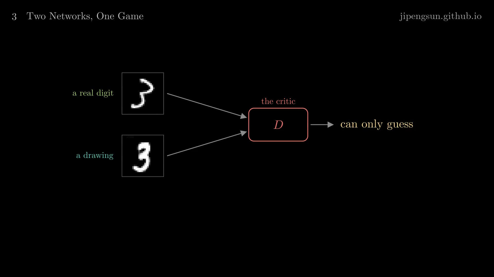
Figure 5. Where the game ends in theory: the drawings are as real as the data, and the critic can only guess.

The theory assumes what practice does not give: a critic that is the best possible at every moment, networks that can represent any distribution, and exact expectations. Real training takes small alternating steps on batches, and three problems follow.

Problem 1: vanishing gradients, and keeping the two balanced

Think of yourself as the generator, a learner, and of the critic as your grader. At the start, the critic wins at once: in our run, ten steps in, it scored real digits 0.995 and fakes 0.02, and until about step 170 it was nearly perfect. It is an easy call: the generator's first drawings are a flat gray, nothing like a digit, and telling the two apart takes a classifier a few steps, while learning to draw takes the generator thousands. For the learner, that is a stack of problems far too hard: every answer comes back wrong, and a bare "wrong" says nothing about what right would look like.

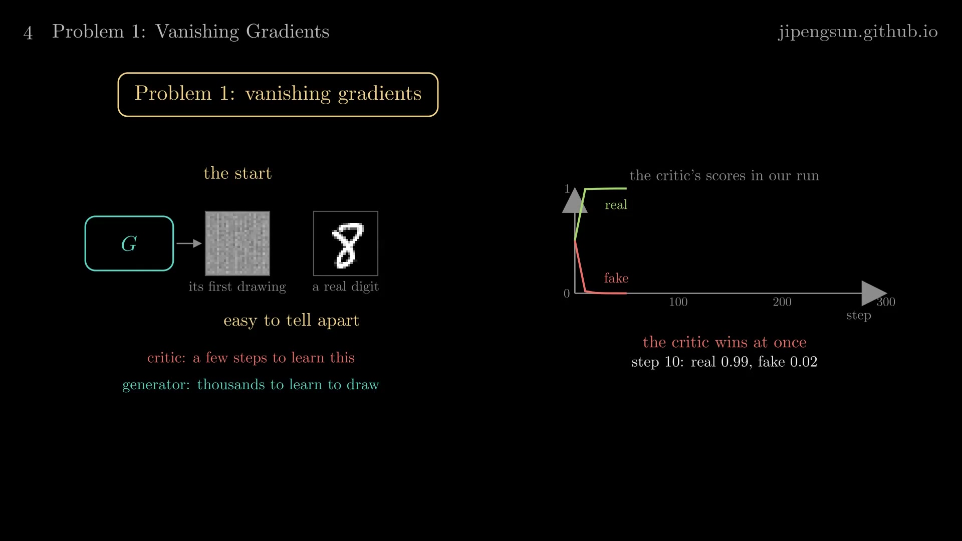
Figure 6. At the start the critic wins at once. The generator's first drawing is a flat gray, easy to tell from a real digit: ten steps in, the critic scores real digits 0.99 and fakes 0.02.

The original generator loss makes this literal. Write the critic's score as \(D = \sigma(s)\), where \(s\) is its raw output (a logit) and \(\sigma\) the sigmoid. The generator's push on a fake comes through \(s\), and

\[\frac{\partial}{\partial s} \log\big(1 - \sigma(s)\big) = -\sigma(s), \qquad \frac{\partial}{\partial s}\Big(-\log \sigma(s)\Big) = -\big(1 - \sigma(s)\big).\]

Where the critic is sure a picture is fake, \(\sigma(s) \approx 0\): the original loss is nearly flat in \(s\) (slope 0.02 at \(D = 0.02\)), so its gradient vanishes, while the non-saturating loss keeps a slope near 1 (0.98). Measured on our generator at step 10, the push, the size of the loss's gradient on each fake's pixels, was 0.0008 with the original loss and 0.64 with the non-saturating one, about 750 times larger. Trained with the original loss, an otherwise identical run still drew static after 2,808 steps, its critic at 1.000 against 0.000 throughout. With the non-saturating loss, the generator caught up within about 300 steps (at step 300 the critic scored 0.82 against 0.32) and drew digits by step 1,000. That is the first fix: keep "wrong" informative, so that even a confident rejection says which way to change.

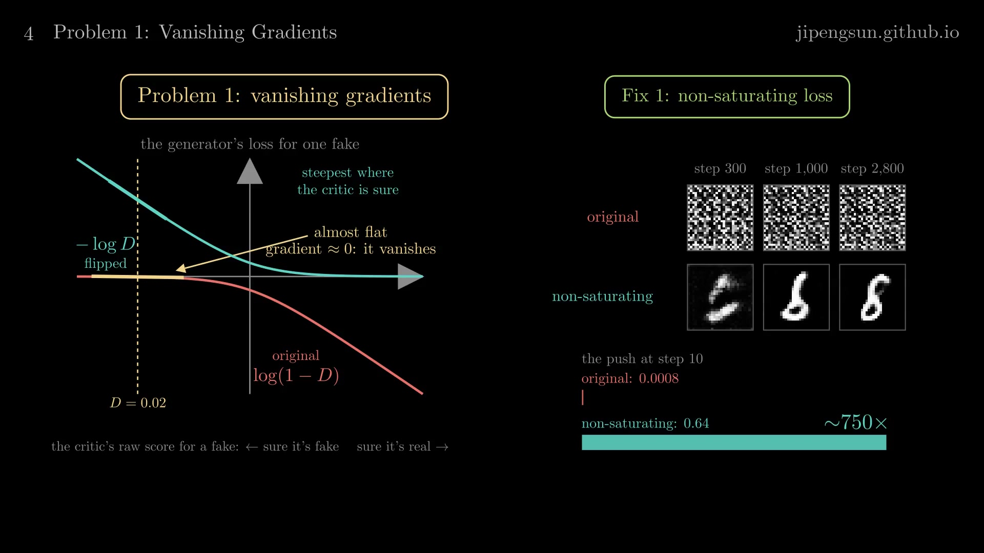
Figure 7. Where the critic is sure a picture is fake, the original loss \(\log(1 - D)\) is almost flat and the flipped \(-\log D\) is steepest. At step 10 the push grows about 750 times, and the same generator draws digits by step 1,000 instead of static.

The second fix is balance, and the learner's view explains it. If the tests stay too hard, all the learner ever hears is "wrong", and nobody shows it the right answer. Given five steps, at twice the learning rate, for each generator step, our critic scored the fakes about 0.10 and real digits 0.93 from step 1,000 on, and the generator fell back on the digits it could fake most easily: at step 2,800, of 100 fixed noises, 40 drew a one and 20 a zero, while 1 drew a six and 2 a two. If the tests become too easy, all the learner hears is "right", and it learns nothing. A critic that stops learning is such a test, and a learner soon games it: frozen at step 1,000, our critic's score for the fakes rose from 0.48 to 0.97 within 600 generator steps, while the fakes turned into blocky patterns that are not digits. Learning happens when each test is a little harder than what the learner can already do. With the same learning rate and one step each, our critic stayed a step ahead, scoring real digits about 0.64 and fakes about 0.37 between steps 1,000 and 2,800, and all ten digits came out clean. The balance is a range, not a knife edge: a critic learning ten times slower, whose scores for real digits and fakes stayed within 0.05 of each other around one half, still taught our generator as fast as the balanced run (at the same steps, a digit classifier read the two runs' drawings with the same confidence, 0.85 against 0.84 at step 1,400). The trouble comes at the extremes.

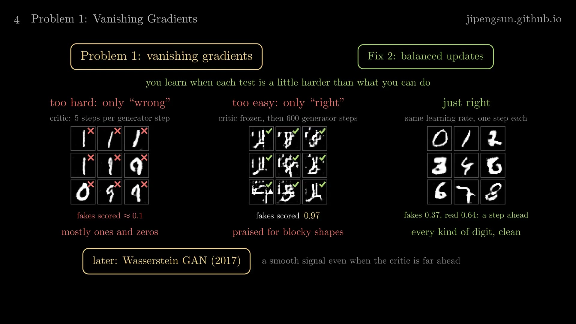
Figure 8. Balanced updates, with the generator as the learner: five critic steps per generator step leave only "wrong" (mostly ones and zeros); a frozen critic leaves only "right" (blocky shapes scored 0.97); one step each keeps the critic a step ahead (every kind of digit).

Later work went further. The Wasserstein GAN (2017) replaces the probability with a score whose slope is kept bounded. That score estimates the Wasserstein distance between the real and generated distributions and keeps giving the generator a smooth, useful signal even when the critic is far ahead. The bound is enforced by clipping the critic's weights, by a gradient penalty, or by spectral normalization.

Problem 2: non-convergence

Even balanced, the game need not settle: each side reacts to the other's last move, and the moves can circle the answer instead of reaching it. The simplest case (Mescheder et al., 2018) has real data at the single point \(x = 0\), a generator that draws a single point \(\theta\), and a critic \(D(x) = \sigma(\psi x)\) that can only tilt, by \(\psi\). The answer is \(\theta = 0\) and \(\psi = 0\). With the original loss and step size \(\eta\), the critic's step is \(\psi \leftarrow \psi - \eta\, \sigma(\psi\theta)\,\theta\) and the generator's is \(\theta \leftarrow \theta + \eta\, \sigma(\psi\theta)\,\psi\). Near the answer \(\sigma \approx 1/2\), so \(\psi\) changes by \(-\tfrac{\eta}{2}\theta\) and \(\theta\) by \(+\tfrac{\eta}{2}\psi\): a small rotation of the pair \((\theta, \psi)\) around \((0, 0)\), not a step toward it. The fake moves toward the higher score, reaches the real point while the critic is tilted hard, overshoots, the critic flips, and the fake swings back. Taking the steps alternately with \(\eta = 0.1\) from \(\theta = 1.5\), our simulation stayed at distance 1.50 from the answer for 1,200 steps, one lap every 147 steps; taking them at the same time, it spiraled out to 2.85. With the non-saturating loss, alternating steps creep inward, but slowly.

Our real run shows the same restlessness. The critic's average scores swing from step to step for all 9,360 steps, and at the end it still scored real test digits 0.55 and fakes 0.28; no loss value tells you training is done. The generator's pictures jitter too. In a second run with the main settings, from step 3,000 to the end, each of 100 fixed noises changed digit (as read by a classifier) 6.7 times on average between snapshots 100 steps apart; one of them read 8, 5, 0, 0, 0, 8, 8, 5, 5 and 3 over steps 7,600 to 8,500.

The fix we use is weight averaging. Alongside the generator, keep an exponential moving average of its weights,

\[\bar\theta_t = \beta\, \bar\theta_{t-1} + (1 - \beta)\, \theta_t, \qquad \beta = 0.999,\]

where \(\theta_t\) are the generator's weights after step \(t\) and \(\bar\theta_t\) their average. Each step moves the average a tenth of a percent toward the current weights, so it blends roughly the last thousand steps (a step's weights count for \(\beta^k\) after \(k\) more steps), and the back-and-forth cancels. The averaged weights are only used to draw; training continues on \(\theta_t\). Drawn with them, the noise above was an 8 at every one of those steps; across the 100 noises, digit changes per noise fell from 6.7 to 0.9, and the pictures moved 10.7 times less per 100 steps. One pixel of that noise had a standard deviation over training of 0.37 under the raw generator and 0.07 under the average. Other fixes target the rotation itself, such as a gradient penalty on the critic, which makes the one-point game converge.

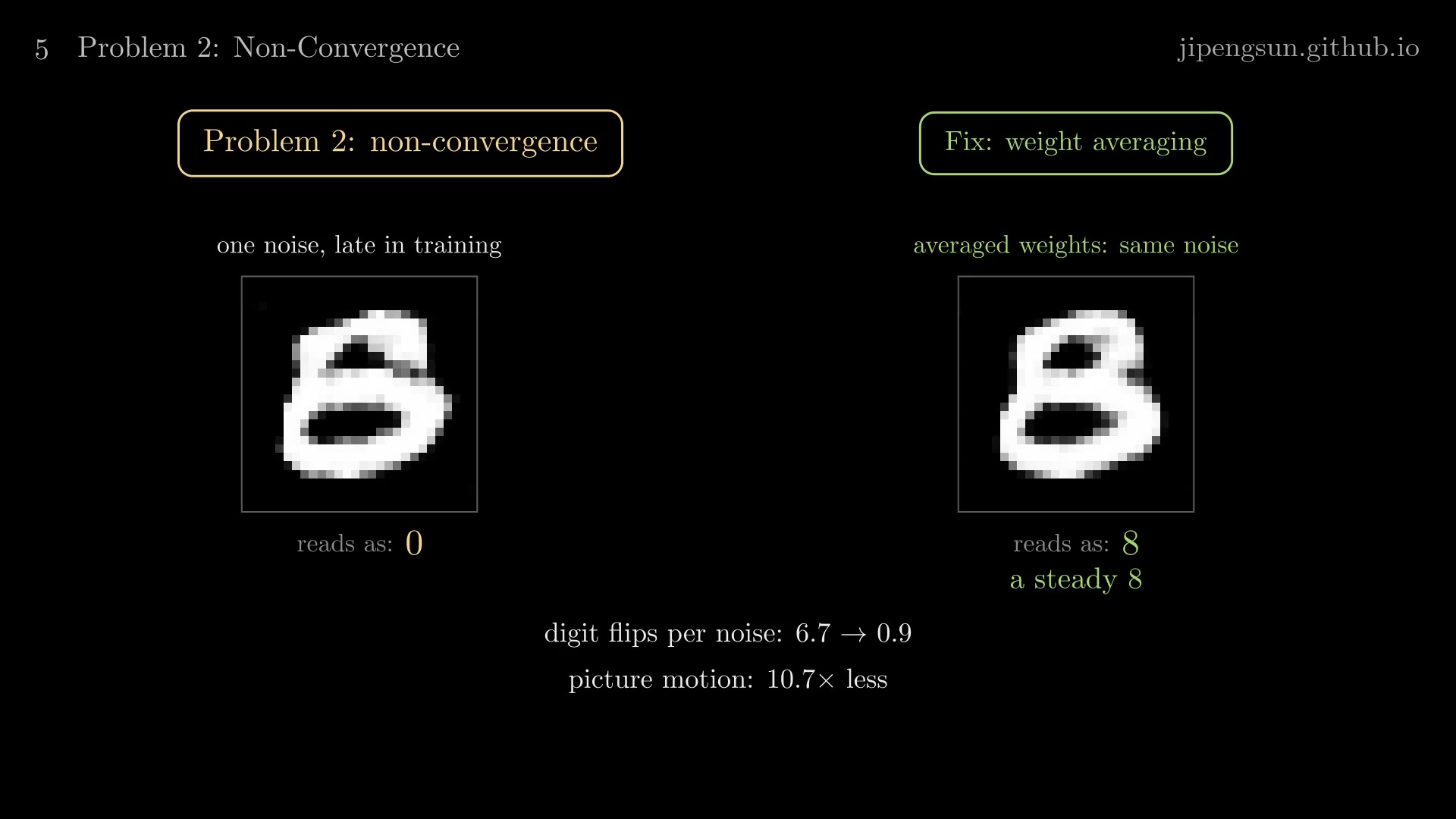
Figure 9. One noise late in training: the raw generator keeps redrawing it (here as a 0), while the weight-averaged generator draws a steady 8. Digit flips per noise fell from 6.7 to 0.9, and the pictures moved 10.7 times less.

Problem 3: mode collapse

Nothing in the generator's loss rewards variety: \(L_G\) scores each fake on its own. Against a fixed critic, the generator's best move would be to draw the one picture the critic scores highest, every time. The critic updates and catches the pile-up, and the pile moves on; because all fakes come from one network, they move together. In a small game with real points in eight tight clusters on a ring (standard deviation 0.02, radius 2; a generator and a critic with two hidden layers of 128 units, 25,000 steps of Adam at \(10^{-4}\) on batches of 512), the fakes sat on one cluster at a time and hopped to another: at step 25,000, 944 of 1,000 were near a single cluster. With digits, a fully connected GAN built the 2014 way (64 random numbers through layers of 256 and 512 units, no convolutions) drew a three for 84 of 100 fixed noises at step 5,000, and over the whole run, 6,100 pictures at 61 snapshots from step 2,000 on, it drew 2,339 threes, 19 sixes and 16 zeros. This is mode collapse: the model covers some of the data's kinds, its modes, and drops others.

Fix one is minibatch discrimination: let the critic look at the whole batch. In its simplest form, the minibatch standard deviation, the critic computes, for each of its hidden features, the standard deviation across the batch, averages these into one number, and appends it as one more input to its last layer. A batch of near-copies has almost no spread, so it is easy to call fake, and the generator has to spread out. In pixels, eight real digits of different kinds spread 0.17 on average, while eight of the collapsed run's threes spread 0.10. With this critic, the same ring game ended with the fakes over all eight clusters, between 92 and 143 of 1,000 near each. On the fully connected digit GAN it was no cure: in 15 epochs the zeros still never appeared, and the sixes rose only from 1 to 28 of 2,600 pictures.

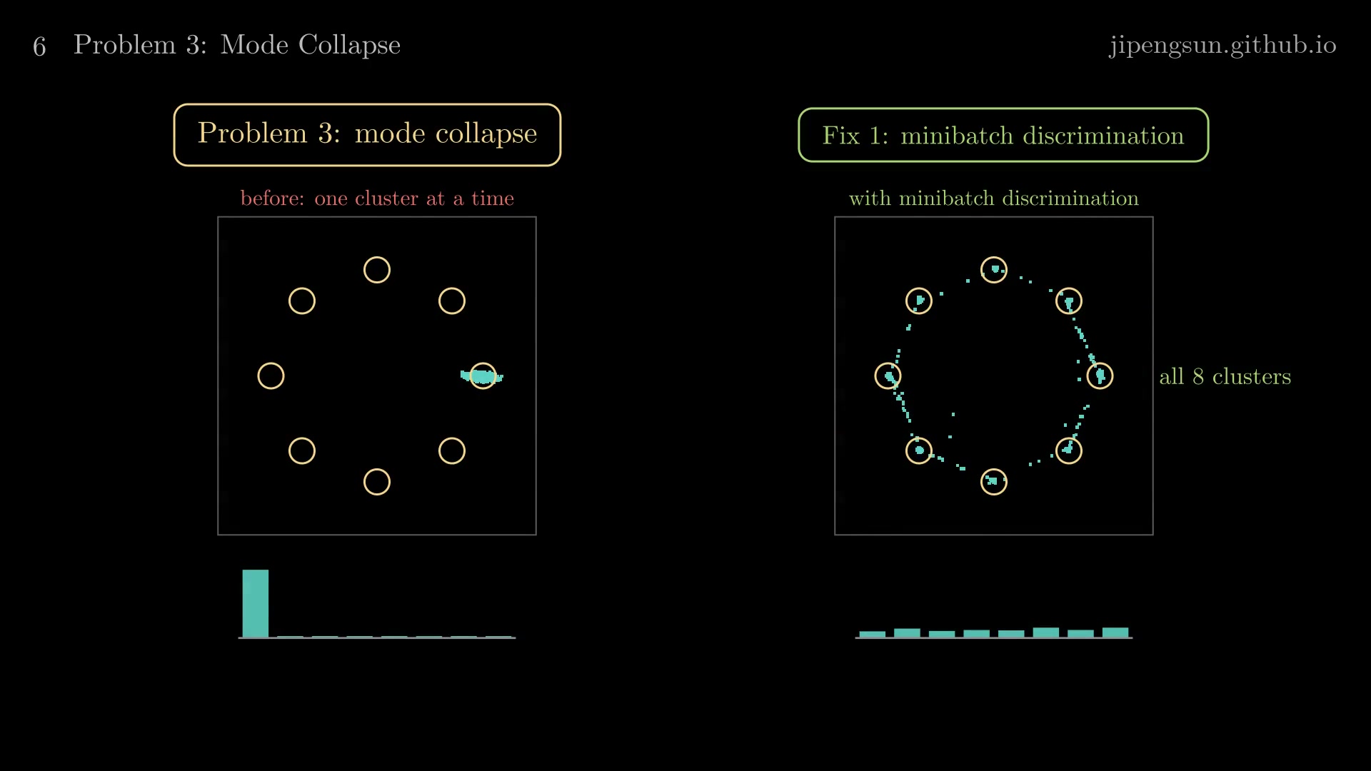
Figure 10. Mode collapse in the ring of eight clusters: the plain GAN's fakes sit on one cluster at a time; with minibatch discrimination they cover all eight.

Fix two is in the architecture: batch normalization in the generator, as in DCGAN (2015). Each normalized layer rescales its outputs across the batch to zero mean and unit spread before a learned scale and shift, which makes it hard to send every noise to the same picture. Without it, our generator and critic collapsed completely: from step 600 on, all 100 fixed noises drew one identical picture. With it, our generator drew all ten digits, though not in equal shares: in 2,000 samples, 68 twos and 79 sixes, against 218 and 170 in 2,000 real test digits. Nothing in the loss guarantees variety; these fixes make collapse less likely, not impossible.

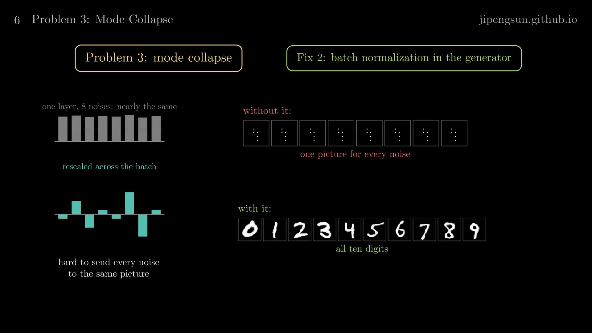
Figure 11. Batch normalization in the generator: without it, every noise drew the same picture; with it, all ten digits.

From a good idea to a practical one

These fixes, and others, made the idea practical: the first GAN and its non-saturating loss (2014); DCGAN's convolutions and batch normalization (2015); minibatch discrimination and other training techniques (2016); the Wasserstein GAN and its gradient penalty (2017); spectral normalization, and the progressive GAN with its minibatch standard deviation and weight averaging (2018); and StyleGAN (2019), whose faces are hard to tell from photographs.

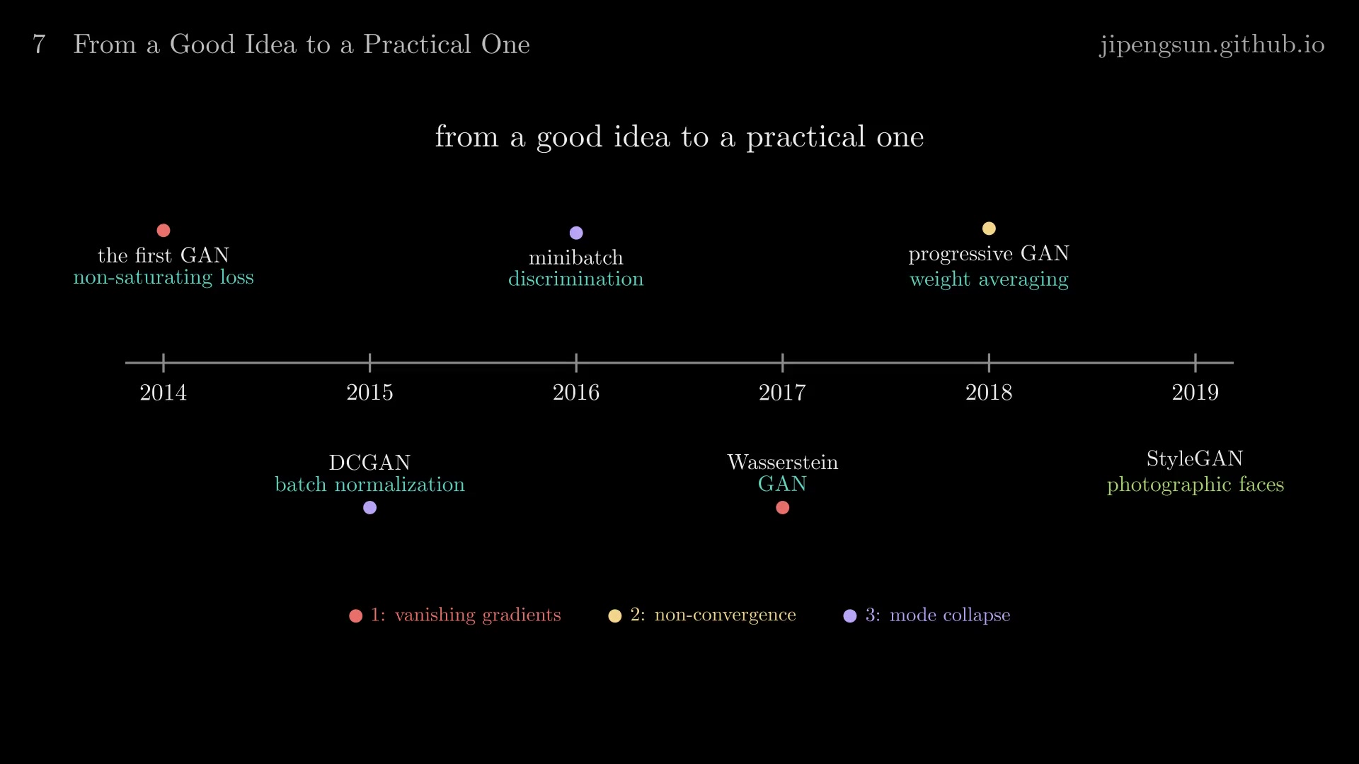
Figure 12. The fixes that made GANs practical, 2014 to 2019, colored by the problem each one addresses.

Compared with the Variational Autoencoder (VAE), which grades each drawing pixel by pixel against an assigned image and so averages where codes overlap, the GAN's learned judge gives sharp pictures in one network pass. Our GAN's samples are 0.96 as sharp as real digits by the mean squared change between neighboring pixels, against 0.31 for the VAE's, and a fresh critic told the VAE's samples from real digits 95% of the time after 30 training steps: a blur is an easy giveaway. The price is the three problems above. Diffusion models, the next method in this series, build an exact answer key instead, by burying real pictures in known noise.

Summary

A GAN trains a generator against a critic that learns to tell its drawings from real data; the critic's labels come free, and its gradient tells every pixel which way looks more real. Against the best critic, \(D^* = p_{\text{data}}/(p_{\text{data}} + p_g)\), the game ends only when the generator's distribution equals the data's, with every score one half. In practice the critic wins too early (vanishing gradients: use the non-saturating loss and keep the two balanced, like a grader a step ahead of the learner), the game circles instead of settling (non-convergence: average the generator's weights), and nothing rewards variety (mode collapse: let the critic see the batch, and normalize the generator's layers). Those fixes turned a good idea into a practical one.