The core premise of this method is to shift the target of generative training from instantaneous velocity (used in standard Flow Matching) to average velocity. This shift mathematically eliminates the need for multi-step ODE solvers during generation, allowing for state-of-the-art 1-step image generation.

1. The Background: Standard Flow Matching

In standard Flow Matching, the goal is to map a simple prior distribution (like noise, \(\epsilon\)) to a complex data distribution (like images, \(x\)).<br>A flow path is defined as \(z_t = a_t x + b_t \epsilon\), where \(t\) is time.

The model learns to predict the instantaneous velocity (the derivative with respect to time), denoted as \(v_t\):

\[v_t = \frac{d}{dt}z_t = a_t' x + b_t' \epsilon\]

To generate an image, you start with noise \(z_1 \sim p_{\text{prior}}\) and use a numerical ODE solver to integrate this instantaneous velocity field step-by-step to reach \(z_0\). Because the trajectories are curved, taking a single large step results in severe inaccuracies.

2. The Innovation: Average Velocity

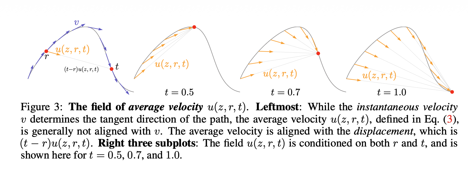
Instead of the instantaneous velocity, the authors define the average velocity \(u\) between two time steps \(r\) and \(t\). It is the total displacement divided by the time interval:

\[u(z_t, r, t) \triangleq \frac{1}{t-r}\int_r^t v(z_\tau, \tau)d\tau\]

If a neural network could perfectly learn this average velocity \(u\), you wouldn't need an ODE solver. You could jump directly from \(t=1\) (noise) to \(r=0\) (data) in a single step. However, training a network directly on this definition is intractable because evaluating the target requires computing the integral over the unknown velocity field.

3. The "MeanFlow Identity" (The Mathematical Trick)

To make this tractable, the authors manipulate the definition of average velocity to remove the integral.

First, they multiply both sides by \((t-r)\):

\[(t-r)u(z_t, r, t) = \int_r^t v(z_\tau, \tau)d\tau\]

Next, they take the total derivative with respect to \(t\) (treating \(r\) as independent). Using the product rule on the left side and the Fundamental Theorem of Calculus on the right side, they get:

\[u(z_t, r, t) + (t-r)\frac{d}{dt}u(z_t, r, t) = v(z_t, t)\]

> This means the instantaneous velocity at t is equal to the average velocity between r and t plus the average velocity’s acceleration multiply by the time interval. i.e. The average speed of the past interval is the instantaneous speed minus the average speed’s change along the past interval, which is v(r) irrelevant.

Rearranging this gives the MeanFlow Identity:

\[u(z_t, r, t) = v(z_t, t) - (t-r)\frac{d}{dt}u(z_t, r, t)\]

This identity is powerful because it expresses the average velocity \(u\) purely in terms of the instantaneous velocity \(v\) and the total time derivative of \(u\). There are no integrals left.

4. Expanding the Total Derivative

To train a network \(u_\theta\) to match this identity, the network needs to compute that total time derivative \(\frac{d}{dt}u\). Using the chain rule, the total derivative of \(u(z_t, r, t)\) is:

\[\frac{d}{dt}u(z_t, r, t) = \frac{dz_t}{dt}\partial_z u + \frac{dr}{dt}\partial_r u + \frac{dt}{dt}\partial_t u\]

Since \(\frac{dz_t}{dt} = v(z_t, t)\), \(\frac{dr}{dt} = 0\), and \(\frac{dt}{dt} = 1\), this simplifies to:

\[\frac{d}{dt}u(z_t, r, t) = v(z_t, t)\partial_z u + \partial_t u\]

This is computationally cheap. It can be computed efficiently using a Jacobian-Vector Product (JVP) in frameworks like PyTorch or JAX by multiplying the Jacobian of \(u\) with the tangent vector \([v, 0, 1]\).

5. The Training Objective

The model \(u_\theta\) is trained using a regression loss to satisfy the MeanFlow Identity. In practice, the marginal velocity \(v(z_t, t)\) is replaced by the sample-conditional velocity \(v_t\) (just like in standard Flow Matching).

The loss function is:

\[\mathcal{L}(\theta) = \mathbb{E} || u_\theta(z_t, r, t) - \text{sg}(u_{\text{tgt}}) ||_2^2\]

Where the target is:

\[u_{\text{tgt}} = v_t - (t-r)(v_t \partial_z u_\theta + \partial_t u_\theta)\]

(Note: \(\text{sg}\) stands for stop-gradient. It prevents backpropagation through the target's JVP calculation, keeping training stable and avoiding higher-order derivatives.)

6. Single-Step Sampling and CFG

Once trained, sampling requires only a single network evaluation (1-NFE). Starting from noise \(z_1 \sim p_{\text{prior}}\):

\[z_0 = z_1 - u(z_1, 0, 1)\]

Furthermore, the paper shows how to bake Classifier-Free Guidance (CFG) directly into the target field equations. Instead of evaluating the network twice during sampling (once with the class condition, once without) and interpolating—which doubles the compute cost—the MeanFlow network directly learns the CFG-adjusted average velocity. This preserves the ability to sample a high-quality, guided image in exactly one function evaluation.

Why there is a stop gradient operation in the loss?

The stop-gradient operator—denoted as \(\text{sg}(\cdot)\) in the paper—is a critical engineering trick. Without it, the model would either crash your GPU from running out of memory or take an incredibly long time to train.

To understand why it is there, we have to look at what happens if we *don't* use it.

The Problem: A Derivative of a Derivative

Here is the loss function from the paper:

\[\mathcal{L}(\theta) = \mathbb{E} || u_\theta(z_t, r, t) - \text{sg}(u_{\text{tgt}}) ||_2^2\]

And here is the target:

\[u_{\text{tgt}} = v(z_t, t) - (t-r)(v(z_t, t)\partial_z u_\theta + \partial_t u_\theta)\]

Notice that our neural network parameters (\(\theta\)) appear on both sides of the minus sign. The network is essentially trying to predict a target that is created using its own internal gradients (\(\partial_z u_\theta\) and \(\partial_t u_\theta\)).

If you omit the stop-gradient, standard backpropagation will try to update \(\theta\) by taking the derivative of the entire loss equation.

Because the target *already* contains first derivatives (\(\partial u_\theta\)), taking the derivative of the target means calculating the derivative of a derivative.

The Cost of "Double Backpropagation"

In deep learning, computing second-order derivatives (often called double backpropagation or calculating the Hessian matrix) is notoriously problematic:

1. Massive Memory Cost: Tracking the computational graph for second-order derivatives requires storing exponentially more intermediate values in VRAM.
2. Extremely Slow: It mathematically turns a fast, linear operation into a highly complex, multi-step calculation.
3. Unstable Training: Second-order gradients are highly sensitive and can cause the optimization landscape to explode, making the loss spike to infinity.

The Solution: The Stop-Gradient \(\text{sg}()\)

The paper applies a stop-gradient to the target. This acts as a circuit breaker for PyTorch's automatic differentiation engine.

When PyTorch sees \(\text{sg}(u_{\text{tgt}})\), it calculates the exact numerical value of the target using the current weights, but then it completely severs the computational graph. It tells PyTorch: "Treat this final matrix of numbers as a fixed, frozen constant. Do not try to trace how we calculated it."

By freezing the target, PyTorch only has to compute the gradient for the left side of the equation (\(u_\theta\)), which is a standard, cheap, first-order derivative.

Implementation

1. What the Network is Actually Learning

The neural network, denoted as \(u_\theta(z_t, r, t)\), is learning to predict the average velocity \(u\) between two arbitrary points in time, \(r\) and \(t\). It takes three inputs:

• \(z_t\): The current noisy image at time \(t\).
• \(t\): The current time step.
• \(r\): A target time step somewhere in the past (closer to a clean image).

By learning this, the network understands how to "skip" from time \(t\) to time \(r\) in a single jump, rather than taking tiny, step-by-step instantaneous movements.

2. How Data is Prepared (Calculating \(z_t\))

During training, the system does not run a simulation; it simply pulls random states from known math formulas.

1. Grab a perfectly clean image from the dataset, \(x\).
2. Generate pure Gaussian noise of the exact same size, \(\epsilon\).
3. Calculate the noisy image \(z_t\) using straight-line interpolation:

\[z_t = (1-t)x + t\epsilon\]

1. Calculate the instantaneous velocity \(v_t\) (the direction from the image to the noise):

\[v_t = \epsilon - x\]

3. Are \(r\) and \(t\) random? (How they are sampled)

Yes, during training, \(r\) and \(t\) are completely random. The goal is to teach the network the average velocity between *any* two arbitrary points on the flow path.<br>Here is exactly how they sample them:

• They draw two random numbers from a specific distribution (they found a "logit-normal" distribution works best, which slightly favors values closer to the middle rather than the extreme 0 or 1 edges).
• They sort them: the larger number becomes \(t\) and the smaller number becomes \(r\).
• The 25% Trick: To keep the network stable, they force \(r = t\) for 75% of the training batches. When \(r = t\), the model acts exactly like a standard Flow Matching model learning instantaneous velocity. For the remaining 25% of the time, they let \(r \neq t\), which forces the network to learn the "MeanFlow Identity" and master large jumps.

4. The Training Process (Putting it together)

For every single batch of images, the training loop runs like this (summarized from Algorithm 1 in the paper):

1. Sample \(r\) and \(t\) randomly (as described above).
2. Calculate the noisy image \(z_t\) and instantaneous velocity \(v_t\).
3. The Forward Pass & JVP: Pass \(z_t\), \(r\), and \(t\) into the network. Because of the PyTorch jvp function, the network outputs both its prediction for the average velocity (\(u\)) AND the total time derivative (\(\frac{du}{dt}\)) simultaneously.
4. Calculate the Target: The ground-truth target is calculated using the MeanFlow Identity:

\[u_{\text{tgt}} = v_t - (t-r)\frac{du}{dt}\]

1. Compute Loss: The network is penalized using a Mean Squared Error (L2) loss between what it predicted (\(u\)) and the target (\(u_{\text{tgt}}\)). A stop-gradient is applied to the target to prevent optimization crashes.

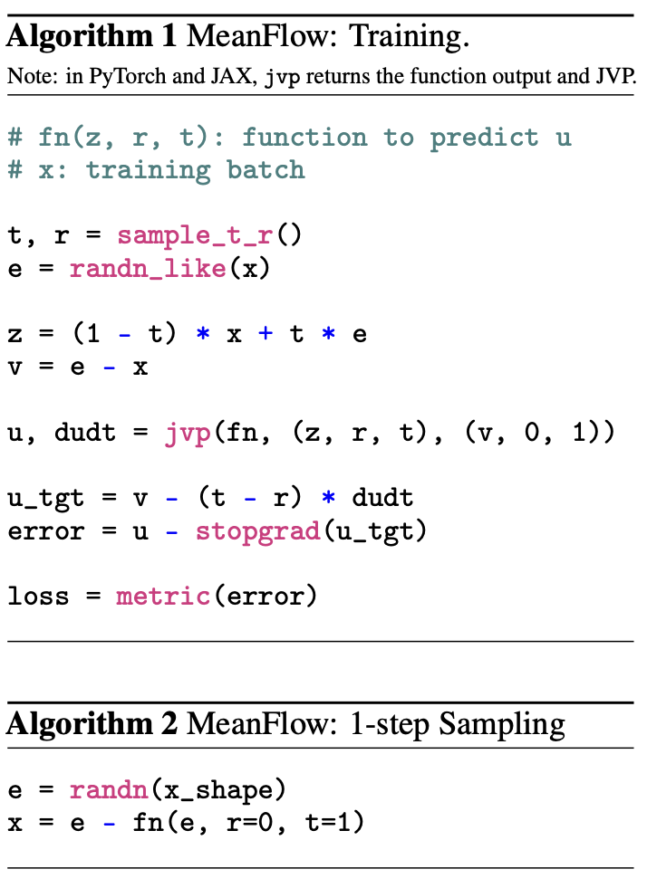
5. How to Sample (Inference)

During sampling, nothing is random except the starting noise. Because the network has perfectly learned the average velocity between any two points, you can just hardcode \(t=1\) (the start of the journey) and \(r=0\) (the end of the journey).

To generate an image in 1 step:

1. Generate pure noise: \(z_1 \sim \mathcal{N}(0, I)\).
2. Ask the network to predict the average velocity spanning the entire process:

\[u = u_\theta(z_1, r=0, t=1)\]

1. Subtract that average velocity from the noise to instantly get your clean image:

\[z_0 = z_1 - u\]